Differentiable Rocket Science
View on GitHub → Updated 2026-07
A neural network learns spacecraft maneuvers by backpropagating through the physics. 92.3% success on the full 3-D task, and 1.03× the analytic-optimal fuel at the best-fuel checkpoint, with the headline circularization numbers re-flown at float64 before they were stated and every other lane checked against its own verification pass.
Abstract
In 2021 I tried to train a reinforcement learning (RL) agent to fly a spacecraft from Earth to the Moon for a graduate astrodynamics course. It trained overnight run after overnight run and never learned anything: the distance to the target went up, not down, no matter what I tried. In 2026 I went back, audited the old code, found the real bugs, and rebuilt the project on a different idea — instead of letting the agent learn by trial and error, differentiate through the physics itself and hand it the exact gradient of fuel cost with respect to its own weights. On a full 3-D orbit-circularization task with quaternion attitude dynamics, the result is a policy that succeeds on 92.3% of 4,096 fresh random orbits. A sibling checkpoint flies the same maneuver at a median fuel cost 1.03× the analytic optimum on a float64 re-flight. It matches the textbook maneuver; it does not beat it — on this problem that maneuver is the standard analytic optimum, so matching is the correct result. In the regimes where the textbook is not optimal, the same method rediscovers a real operational technique (J2 nodal-drift phasing) from the raw objective, discovers combined burn maneuvers on its own, and achieves a verified ballistic lunar capture — arrival in orbit around the Moon without a capture burn. On a differentiable model of the real solar system, it also finds the gravity-assist strategy for changing orbital planes on its own: crank inclination up to the kinematic ceiling arcsin(v∞/v_P), and pump the flyby excess speed to lift that ceiling. The tour it discovers runs against the real ephemeris, four pumping flybys and then a crank walk, and it hits every encounter ballistically: excess speed 5.95 → 16.3 km/s, then inclination to 97% of the ceiling (92% counting only the tightly-closed legs). Every circularization claim comes from a fresh evaluation set and survives a float64 re-flight, an integrator energy audit, and a check that no episode gamed the success tolerance; the multi-body and low-thrust results carry their own verification (dt-robustness, conserved-quantity audits, and analytic cross-checks). All code, the round-by-round experiment records in the repo docs, and the original 2021 failure are public.
1. The course project that didn't work
This started as a final project for a graduate astrodynamics course in 2021: train an RL agent to find an optimal Earth-to-Mars trajectory under real N-body gravity, and compare it to the Hohmann transfer every textbook derives. I scoped it down to Earth-to-Moon when I realized a single Mars episode would take days to simulate. Then I spent weeks watching it fail.
The final report I turned in was honest about the outcome:
"Due to the complexity of the project, and the time constraint imposed, it appears I have bitten off much more than I could chew."
The symptom was always the same. The agent's score improved as it trained, but the distance to the Moon steadily increased. The spacecraft spent most of its episodes flipping its own orientation back and forth — two of the four discrete actions it could choose were orientation changes, and it used them constantly without going anywhere. An episode is one simulated flight, start to finish.
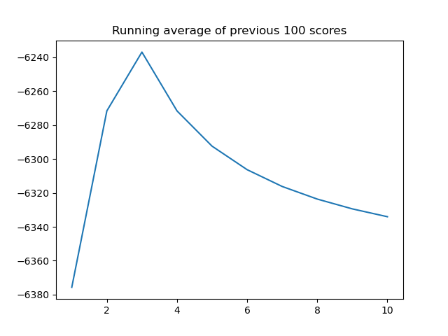
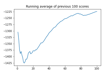
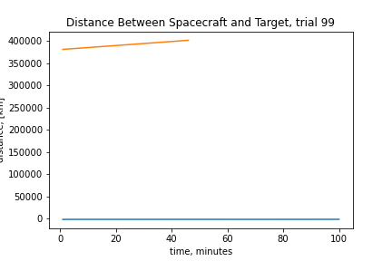
That's a training curve going up while the thing you actually care about goes nowhere. I blamed the reward function, my unfamiliarity with Python, the size of the observation space, and the training time. Some of that was right. But one paragraph in that report mattered more than everything else in it. It described a reward function I ran out of time to try, one that would reward the agent for tracking a precomputed transfer ellipse:
"However, this approach begs the question: if such an orbital path can be defined in the first place, what use is it to utilize a RL agent to follow the path? The entire point is to see if the optimum path can be learned without such direct supervision and guidance."
That question became the design rule for the whole revival.
2. The problem
Take a spacecraft in a stretched-out elliptical orbit around Earth. You want it in a clean circular orbit, and you want to spend as little fuel as possible. Fuel spent is measured in delta-v (Δv) — the total change in velocity your engine produces.

Every orbital mechanics student learns the answer. Coast to apoapsis — the high point of the ellipse, where you're moving slowest — and burn prograde (in the direction of travel) until your speed reaches circular speed. Burn anywhere else, or point the wrong way, and you pay more.
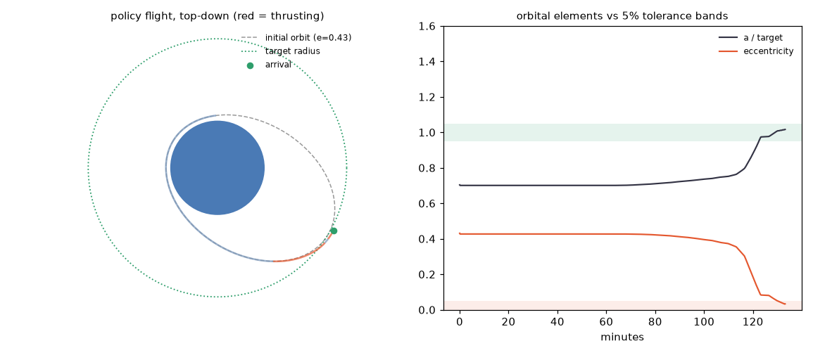
That is one episode flown by the trained policy: the network itself, the rule that turns what the spacecraft sees into what it does next. Red segments are burns, blue is coasting. The right panel carries the two numbers that define success: semi-major axis ratio and eccentricity, both of which have to land inside a 5% tolerance band and stay there. The semi-major axis is half the ellipse's long diameter, so the ratio is the orbit's size against the size it is meant to be. Eccentricity is how squashed it is, and 0 is a circle.
The concrete task, in both the 2-D and 3-D versions:
| Element | Value |
|---|---|
| Dynamics | Two-body gravity around Earth (gravitational parameter μ = 398,600.4418 km³/s²), integrated with RK4 (fourth-order Runge–Kutta) |
| Start orbit | Random ellipse: periapsis (the low point) at 400–800 km altitude, apoapsis/periapsis ratio 1.3–2.5, random entry point; in 3-D also random inclination ≤ 40° and random initial attitude |
| Goal | Circular orbit at the initial apoapsis radius, within 5% on semi-major axis and eccentricity |
| Budget | 2.0 km/s of Δv |
| Yardstick | The analytic single-impulse circularization burn at apoapsis — the textbook optimum for this maneuver |
The yardstick is worth one absolute number. Across the sampled orbits the analytic apoapsis burn costs 0.44 to 1.18 km/s, a median of about 0.93, and the spacecraft is moving 3.6 to 6.3 km/s when it makes that burn. The 2.0 km/s budget is roughly twice the median optimal burn. Fuel in the circularization results is quoted as a multiple of that burn: 1.00× is the analytic single-impulse cost, and anything under it wants explaining rather than celebrating. Later results priced against a different baseline name the baseline they use.
Why circularization and not Earth-to-Moon? Because it's the smallest problem that still contains the hard parts — burn timing, burn direction, attitude control, fuel accounting — and it has a closed-form optimal answer to measure against. The interplanetary goal is Section 11. In 2021 I started with the hardest version of the problem and learned nothing from the failures. This time the plan was to earn each level of difficulty.
The analytic yardsticks are implemented in the repo alongside the simulator: the single-impulse apoapsis circularization, the two-burn Hohmann transfer, and the three-burn bi-elliptic transfer (which can beat Hohmann once the radius ratio exceeds 11.94, and always beats it above 15.58 — the first hint that "the textbook answer" is a set of special cases).
3. The autopsy
Before rebuilding anything, I got the 2021 code running again, exactly as it was. It reproduced the original failure on the first try: distance to the Moon increasing monotonically, 379.9 to 393.8 Mm over an episode, episodes never terminating. Reproducing your own failure five years later is a strange kind of satisfying.
Then I audited the code line by line. The 2021 report blamed the reward function and the training time. The audit found the actual bugs, and they were worse:
| Finding | Detail |
|---|---|
| Discrete agent, continuous world | The PPO (Proximal Policy Optimization) implementation output a single integer from a softmax — it was built for discrete actions. The environment expected continuous roll/pitch/yaw/throttle commands. The two halves were never reconciled. Coherent learning was impossible from the start. |
| The reward was a constant | In the second version of the code, getReward() literally returned reward = 1, and checkDone() returned False. No learning signal, episodes that never end. |
| Learning rate = 2 | The learning rate is how big a step the optimizer takes on each update. Adam's was set to 2. The Adam paper's own recommended default is 0.001, and 0.0003 is the usual default in deep RL. It was also the default in this code's own Agent class, which mainPPO overrode. And n_games = 1 — a single training episode. |
| Save/load existed but was never called | The report complained that training couldn't be continued across runs. The save/load code worked fine. The call was commented out. |
There were more (reward computed before the action was applied, the reward leaking into the observation, degenerate observation bounds), but those four are the story. The 2021 failure was a discrete plug in a continuous socket, a reward stub some idiot (me) forgot to fill in, and a learning rate four orders of magnitude too hot.
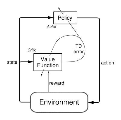
I'm keeping the 2021 code, plots, and reports in the repo permanently. They're the "before" picture, and the audit is reproducible against them.
4. Don't imitate the textbook
The line from the 2021 report — if you can already define the optimal path, what use is it to learn to follow it? — sets the design rule for the revival:
Analytic solutions are yardsticks, never training targets.
You could train a network to imitate the apoapsis-burn maneuver directly. That is behavior cloning, and it runs as one of the four methods in the bake-off. But an imitator can at best match its teacher, and it inherits every assumption the teacher makes. The Hohmann-type analysis is the most efficient two-impulse transfer between coplanar circular orbits, and optimal only under that narrow set of assumptions: two-body gravity, instantaneous burns, moderate radius ratios. Relax any of those and better solutions are known to exist — bi-elliptic transfers, combined-plane-change burns, low-thrust spirals, and multi-body ballistic capture routes that have actually been flown (the Hiten mission reached the Moon that way in 1991). Ballistic means the engine is off and gravity does the work, so the fuel bill for that arc is zero.
Does the textbook maneuver come out on its own when you optimize actual fuel spent through actual physics? And does something better come out in the regimes where the textbook isn't optimal? To keep those questions honest, the agent is never given the analytic maneuver as a training target. The only analytic quantity in the loss is a smooth Δv-to-go shaping term, and the closed-form optimum it is scored against is applied only afterward.
One more design decision, in the same spirit of not repeating 2021: the network makes decisions. Every 200 seconds it outputs a desired thrust direction and a throttle setting, and a deterministic controller does the flying, slewing the spacecraft to the commanded attitude at a bounded rate. Burn planning is learned; burn execution is classical control. The 2021 agent spent its episodes flipping around in space because it was allowed to command rotations directly. This one can't.
5. Four ways to train it
The 2-D version of the task became the bake-off arena. Same environment, same evaluation (success rate over held-out random orbits, and Δv as a multiple of the analytic optimum), four training methods. Held-out means the evaluation orbits were never used in training.
First, a check that the task is solvable at all: a hand-coded scripted controller — coast to apoapsis, latch, burn prograde — solves 100% of seeds (each seed is one randomly drawn start orbit) at 1.00× the analytic Δv. The environment is fair, and every learning method in the table is trying to reach what the script proves is reachable.

| Method | Success | Δv vs optimal |
|---|---|---|
| Scripted expert (hand-coded) | 100% | 1.00× |
| Model-free PPO, from scratch (8 runs) | 0–3% | ~1.1× on the rare success |
| Behavior cloning of the expert | ~16% | ~1.37× |
| DAgger (Dataset Aggregation: cloning + on-policy relabeling) | ~45% (peak 48.5%) | ~1.5× |
| Differentiable-sim policy gradient | 81% | 1.26× |
Model-free PPO fails the way 2021 failed, this time with correct code. The reward for circularizing is essentially zero until you've done most of the maneuver correctly — burn at the wrong point and you've spent fuel making your orbit worse. Random exploration almost never stumbles into "coast for forty minutes, then burn precisely prograde." Eight runs, and the best one solved 3% of orbits.
Behavior cloning collapses off the expert's path. It imitates well on the states the expert visits, then drifts somewhere the expert never went, and has no idea what to do there.
DAgger fixes the drift and hits a different wall. It asks the expert to relabel the states the student actually visits, which did fix the drift. Success stuck at ~45% anyway, while the imitation loss kept improving (0.0115 down to 0.0039). That gap between "imitating better" and "not succeeding more" is structural. The expert is history-dependent: it latches once it reaches apoapsis and stays committed to the burn. The student is a feedforward network with no memory, so it smooths over that sharp decision boundary, and no amount of imitation fixes that.
Exploration can't find the maneuver, and imitation can't represent the teacher. Neither method uses the fact that the dynamics are known: gravity here is a differentiable function I wrote myself.
6. Backprop through the physics
The idea: instead of estimating a training signal from sampled rewards the way RL does, run the whole episode inside an automatic-differentiation framework and compute the loss (how far from circular you ended up, plus every m/s of Δv you spent). Then take its exact gradient with respect to the network weights, backpropagating through every one of the ~1,200 physics steps in the rollout.
A weight is one of the numbers inside the network. There are 18,820 of them here, counting the three weight matrices and the bias vector on each layer, and what the spacecraft sees is pushed through those numbers to decide what it does next. The gradient answers one question about every weight at once: nudge this one up by a hair, and that loss moves this far, in this direction. That is 18,820 slopes, one per weight, and training is a step down each of them. Reinforcement learning estimates that list from sampled outcomes. Differentiating the simulator computes it.
The physics engine is the training signal. If burning 0.4 seconds earlier would have saved fuel, the gradient says so, exactly. Two-thirds of the usual RL machinery — exploration noise and a critic estimating value from samples — drops out entirely. Potential shaping stays, because the raw objective is still too flat to descend. The agent gets told, analytically, how each weight in its network moved the fuel bill.

The pieces, concretely:
- The policy is small. A 13 → 128 → 128 → 4 MLP (multilayer perceptron, a plain feedforward network): three weight matrices you can look at. The 13 inputs are the normalized position and velocity, three orbit errors (semi-major axis, eccentricity, and radius), where the thrust axis currently points relative to the orbit frame, and remaining fuel. The 4 outputs are a thrust direction in the orbit frame (prograde/normal/radial components) and a throttle.
- The controller is not learned. A proportional pointing law slews the body toward the commanded direction at a bounded rate (0.05 rad/s max). Slewing takes real time, so when the policy commits to a burn still matters. The attitude physics stay in the simulation; they are not the network's job.
- The physics is the full 13-state rigid body. Position (3), velocity (3), attitude quaternion (4 numbers for which way it points, and no gimbal lock), angular rate (3), integrated with RK4 at dt = 10 s. The policy decides every 20 substeps (200 s).
- Everything is hand-rolled. The quaternion algebra, the dynamics, the orbital elements, the controller, the environments — all written for this project, typed, and test-covered. No Basilisk, no poliastro. The training hot path is a self-contained re-implementation of that same stack in a differentiable framework, so the fuel gradient flows through the whole rollout, RK4 included.
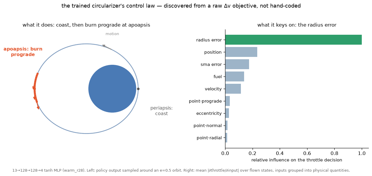
Those three matrices are the whole policy, but reading the raw weights tells you nothing. What matters is the control law they encode, and you can read that straight off the trained network. Sample its commanded thrust all the way around an orbit and it coasts, then fires a prograde burn at apoapsis (left). Ask which of the 13 inputs actually moves the throttle — the mean sensitivity of the throttle to each input over flown states — and the radius error dominates, at four times the next input (right). Nobody wrote that rule down. From a raw fuel objective, the network rediscovered the textbook apoapsis-circularization burn and learned to trigger it on how far it is from the target radius.
In 2-D, this method hit 81% — nearly double DAgger — and its peak checkpoints reached 91% within about a hundred gradient steps. Not a hundred thousand. A hundred. When the gradient is exact, you don't need many of them.
7. Fifty times faster
Backprop through 1,200 physics steps is expensive. The PyTorch implementation took 13.3 seconds per training iteration even after a round of kernel fusion. That is about ninety minutes per debugging cycle.
Porting the hot path to JAX — the rollout compiled through XLA (Accelerated Linear Algebra, the open-source ML compiler JAX targets) with lax.scan, gradients via jit(value_and_grad) — brought that to 0.265 seconds per iteration on the same consumer GPU (an RTX 3060). Fifty times faster, numerically exact against the torch reference: a single RK4 step agrees to 6×10⁻⁸, and the derived orbital elements agree bit-for-bit.
The research loop went from ninety minutes to ninety seconds, and the forensic campaign that followed happened in days instead of months.
8. The hard part: gradient monsters
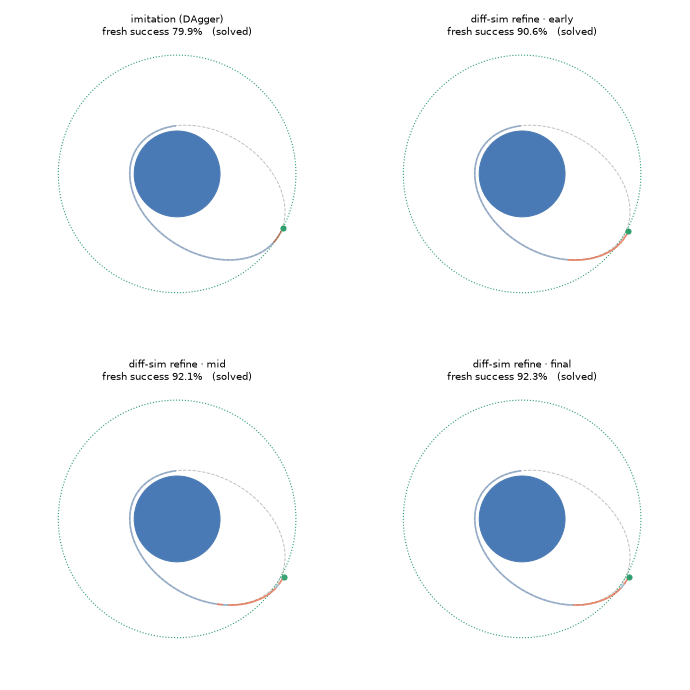
The 3-D campaign started from imitation: DAgger a scripted 3-D expert into the network to get a competent starting policy (79.9% on the fresh evaluation set). The differentiable-sim gradient then refined that policy on the true objective. The plan was for the exact gradient to polish the imitator past its ceiling.
Instead, training collapsed repeatedly.
The cause took a measurement campaign to pin down: gradients that flow backward through a thousand steps of orbital mechanics are heavy-tailed. The norm is a single number for the size of the whole gradient. The median per-episode gradient norm was a few hundred. The 99th percentile reached 10⁸. And a few episodes per few hundred produced finite-but-monstrous norms of 10¹²–10¹⁹. One near-zero commanded thrust direction is enough: the normalization d/‖d‖ has gradient 1/√ε, ~10⁶ at the default ε, and a coasting policy sits there every step, so the product of a thousand Jacobians blows up. One Adam step on one monster and the policy forgets how to fly: measured, a single step at learning rate 5×10⁻⁵ typically moves fresh-set success by ±3 points, and in the tail, −12 points.
I ran the whole campaign as pre-registered rounds: write the hypothesis down, define the measurement, run it, log the verdict. The refutations are written up in the repo's roadmap alongside the survivors; the raw round-by-round logs stayed local.
The playbook that survived is boring and effective: measure the norm distribution, delete the monster tail (trimmed mean over episodes), clip the survivors at the measured 90th percentile, bank progress with an exponential moving average (EMA) of the weights, and polish at low learning rate. No single trick worked alone. Here are four training runs from the same lineage and the same seed: three start from the same checkpoint and differ only in how the per-episode gradients are aggregated, and the fourth is the low-learning-rate polish that follows the winner:
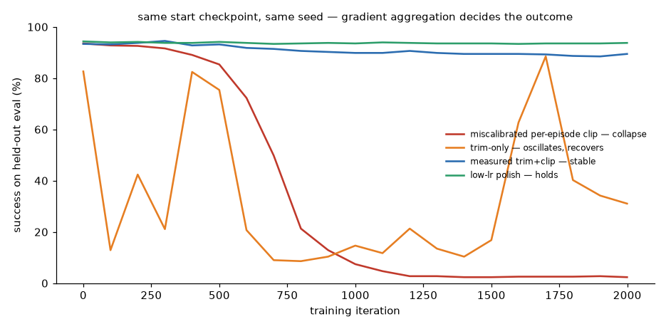
The red run's aggregation was miscalibrated and it collapsed. The blue run's was measured from the actual norm distribution and it climbed.
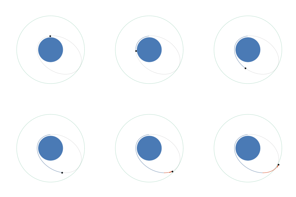
And the payoff on a single episode — the same start orbit flown at four stages of training, the path tightening onto the target ring:
9. Verified results
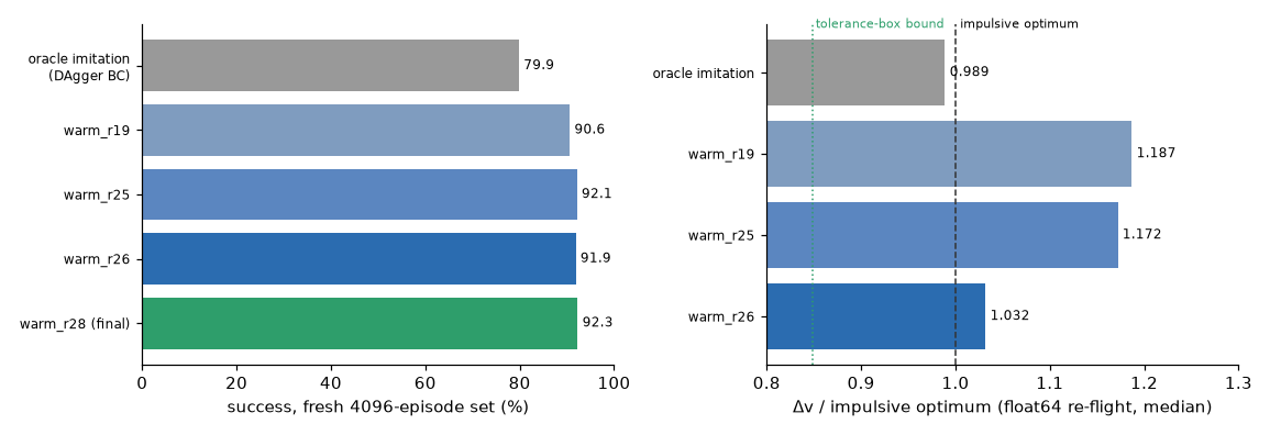
On a fresh 4,096-episode evaluation set (never touched during training):
| Policy | Success | Median Δv vs impulsive optimum |
|---|---|---|
| Imitation oracle (DAgger, the starting point) | 79.9% | 0.989× |
| Best-success checkpoint | 92.3% | ~1.17× |
| Best-fuel checkpoint | 91.9% | 1.032× |
(The oracle's 0.989× is not "beating the optimum" — it succeeds on an easier 80% of orbits and fails the rest, and the tolerance box admits finishes slightly cheaper than exact circularization.)
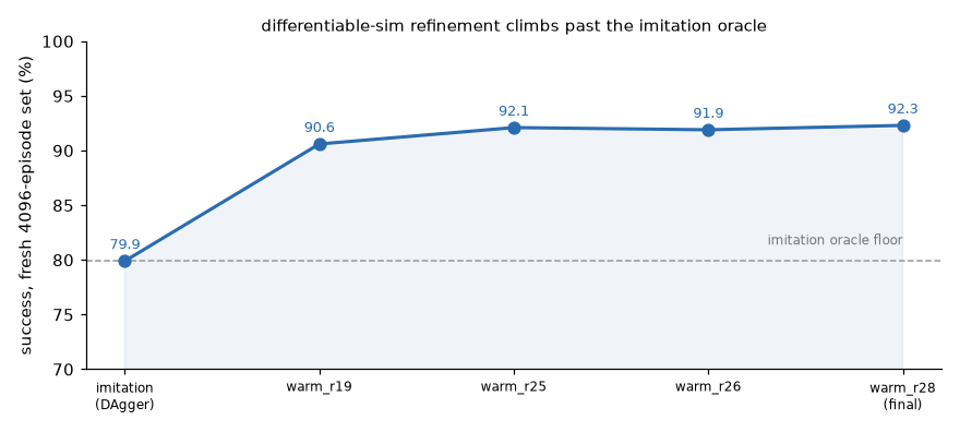
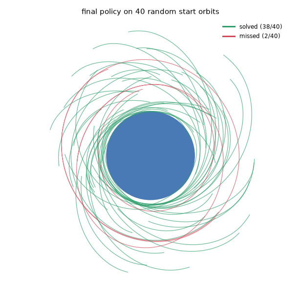
The refinement climbs past the oracle it started from, 79.9% to 92.3%. That gap is what optimizing the true objective buys over imitating a teacher. And it isn't one lucky episode; forty random start orbits flown to termination, colored by outcome:
In 2021 I trusted a rising score and got nothing. This time every headline number passes through a verification harness before it gets stated:
- Fresh data only. All numbers come from evaluation sets generated after training. In-run telemetry is banned from claims — one Adam step can move success ±3 points, so quoting your best in-run number is quoting the winner's curse.
- Float64 re-flight. Float64 is double-precision arithmetic against the training sim's single precision, so rounding can't be what produced the number. Every fuel number in the circularization results is re-flown at float64 with dt = 1 s over a fresh 1,024-episode set, with crashed episodes excluded. The numbers come from that re-flight, not the training sim.
- The sim isn't being gamed. The 5% tolerance box admits solutions about 0.849× the exact circularization Δv at the median. Zero of the 1,024 float64-re-flown episodes finished below their own box bound — the policy isn't exploiting the tolerance.
- The integrator isn't lying. An RK4 energy audit bounds integration error at 0.005–0.02 m/s of Δv-equivalent per episode — more than three orders of magnitude below the differences being claimed.
Put through those four checks, the agent matches the analytic optimum and does not beat it. On this problem, that's the correct outcome — single-body coplanar circularization is exactly the regime where the textbook analysis is the accepted analytic optimum, so matching it is a correctness check on the whole method. The regimes where beating is possible are in Section 11.
10. One network, many missions
Everything so far is one policy trained for one maneuver at its own apoapsis. Several follow-up studies pushed on the "one" part.
Commanded target radii. Ask the headline policy to circularize at a radius other than its own apoapsis and it collapses — about 18% success once the target leaves the radius it trained at. Three attempted in-place fixes failed. The fix that worked was embarrassing in hindsight: the specialist had been cloned from an expert that only ever flew fixed targets, so it had never seen tracking behavior. A target-conditioned scripted expert (drive both apses to the commanded radius) DAgger'd into the same 13→128→128→4 network reaches ~99% success across commanded radii spanning ±15% of apoapsis. The blocker was the imitation source, not network capacity.
Thrust levels. Retrain the policy at lower and lower thrust (a 25× drop, from chemical-engine scale toward electric-thruster scale) and success degrades gracefully, 92% to 77%, while the gravity-loss penalty of long finite burns grows just as the physics predicts (1.20× to 1.38× the impulsive bound). The lowest-thrust specialist flying one episode:
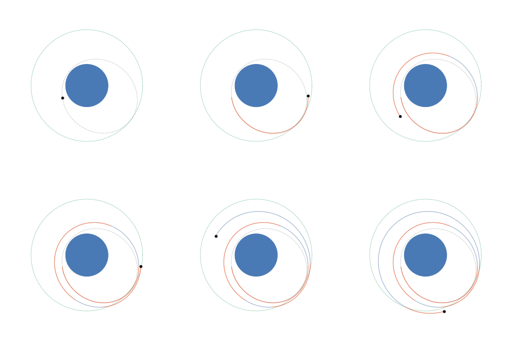
At chemical thrust this maneuver is one short burn at apoapsis. At 25× less thrust there is no crisp burn to make: the policy burns for much of the episode (red), smeared across multiple revolutions, spiraling out to the target circle. But a policy trained at one thrust level craters at another. A single thrust-conditioned generalist — one 14-input network, thrust added to the observation — recovers ~97% of the five specialists' aggregate success (82.1% vs 84.3%). Getting there required distillation + DAgger; differentiable-sim fine-tuning alone left the new thrust input dead. Same lesson as the target study: the gradient refines behavior that exists, but new conditioning enters the network through imitation.
Recovering the classical results. In an orbit-averaged low-thrust model, a policy minimizing raw Δv recovers the Edelbaum spiral, the closed-form optimal low-thrust transfer from low Earth orbit to geostationary orbit (LEO to GEO), at a median 1.006× the analytic value. The LEO-to-GEO case at 28.5° comes out 6.02 vs 5.95 km/s, a ratio of 1.01. And asked for a pure plane change, it rediscovers the raise-turn-return trick on its own: lift the orbit ~10–20%, rotate the plane up high where velocity is small, come back down. That matches the Edelbaum optimum (0.997×) and beats the naive constant-altitude strategy by 4–7%. It found the continuous version of the bi-elliptic inclination trick from nothing but the fuel bill — though only after the yaw parameterization was widened; the first version clamped yaw to ±90°, which silently forbids the return leg.
11. Where the textbook isn't optimal
Here the 2021 question — is the textbook maneuver actually optimal, or just optimal under its assumptions? — finally gets an answer. Three results, in increasing order of how much they mattered to me.
The agent discovers combined maneuvers. Give it an inclined ellipse and ask for a circular and equatorial orbit. The naive approach circularizes, then fixes the plane in a separate burn. The known-better approach folds both into a single combined burn at apoapsis. A diff-sim (differentiable-simulation) policy minimizing raw Δv, with no maneuver structure baked in, reaches 84% success at a median 0.75× the naive two-maneuver cost — right at the analytic combined-burn optimum (1.05× that bound). It's the project's first learned result that beats a reasonable strategy a mission designer might write down, and it found the combined burn without being shown one.
A verified ballistic lunar capture. In the circular restricted three-body problem (CR3BP — Earth and Moon both pulling on the spacecraft, the idealized version of real Earth–Moon dynamics), there exist trajectories that arrive at the Moon already captured — negative Moon-relative energy, no capture burn — threading in along the stable manifold of an orbit around the L2 Lagrange point. Finding them is hard: a straightforward search over departure burns found direct arrivals but zero ballistic captures (that null is logged too — the thin capture set eludes grid-and-gradient search). Building the dynamical-systems machinery — Lyapunov orbits via differential correction, their monodromy matrices, the stable manifolds — and seeding from the manifold produced a verified temporary ballistic capture, and a two-impulse transfer patched onto that manifold beats a steel-manned Hohmann-plus-minimal-capture to the same verified captured state by ~5% (0.18 km/s). Modest, temporary (a couple of weeks bound, in a loose high lunar orbit), and real — in the pure CR3BP, no Sun.
Then the learned policy caught up: backpropagating a two-burn control through the CR3BP rollout achieves its own dt-robust verified capture, staying bound for ~9–10 lunar revolutions (~35 days). The one-burn search had stalled there: across the departure grid it searched, no single burn produced a captured arrival. En route, two reward hacks were caught and fixed — naive "get close to the Moon" objectives get exploited into fast suicidal plunges that technically minimize distance. It's the same class of reward hacking that sank the 2021 project; this time the verification caught it.
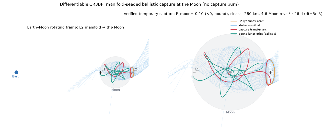
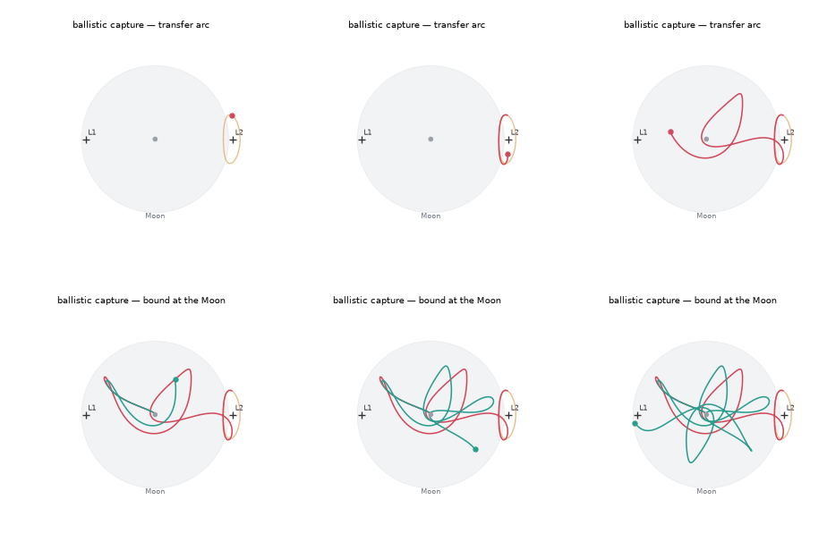
The headline arc in the figure arrives captured and stays bound for 4.6 lunar revolutions — about 26 days — with no capture burn, verified at fine timestep. In this regime the two-body textbook analysis doesn't apply at all.
The J2 story, including the correction. Earth isn't a sphere; its equatorial bulge (the J2 term in the gravity model) slowly rotates every orbit's plane, faster at lower altitude. The textbook impulsive plane-change is blind to this. A diff-sim policy minimizing true Δv over J2-on dynamics, given no maneuver structure at all, rediscovered the operational mechanism used to fan out satellite constellations: change the semi-major axis so J2 drives the node faster, then come back. The altitude-for-nodal-drift trade is standard; the repo's own analytic version of the round trip is what the policy is scored against. It reaches the target plane orientation (the "node") for ~0.88× the cost of passively waiting at a 30° node change, improving to a quarter-to-half of passive at 60–90°. Waiting is not free in Δv: the passive baseline coasts at the starting altitude, lets J2 drift the node on its own, and stops at whichever moment inside the same time budget leaves the least error to clean up. It then pays an impulsive burn for that leftover, and the leftover burn is what the ratios are against.
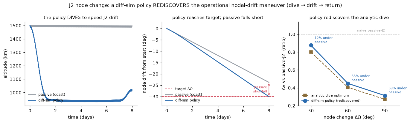
I initially logged this as the project's first genuine beat of a physics-aware strategy. A follow-up round built the analytic version of the same dive-drift maneuver and optimized it directly — and the analytic dive is 8–14% cheaper than the learned one. So the honest classification is rediscovery, not a beat: the agent independently found a real operational technique from the raw objective, and a human with the same insight still executes it better. Both the original claim and the correction are in the repo history.
12. Gravity assists, and a ceiling the agent finds
Everything so far happens near one body. The last thread flies through the whole solar system. The differentiable engine from the ephemeris to-do item now exists: a rollout under many point-mass bodies whose positions come straight from JPL Horizons, with the fuel gradient still flowing through every RK4 step. Before trusting it, I check it against cases with known answers. The two-body Kepler limit closes to one part in 10¹², energy holds to a few parts in 10¹⁵, and from a cold zero-thrust start the optimizer recovers the analytic Lambert transfer to one part in 10¹¹.
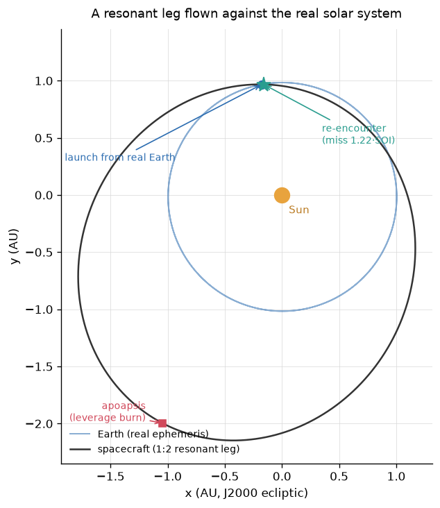
The physics worth flying here is gravity assists: stealing orbital energy and turning the orbit's plane by flying past a planet, for free. Turning a plane with an engine is expensive; a flyby does it for almost nothing, and there is a clean law for how far it can go. The reachable inclination from flybys alone is arcsin(v∞ / v_P) — set by the spacecraft's excess speed past the planet (v∞) and the planet's own orbital speed (v_P), and independent of the planet's mass. That excess speed is what the spacecraft has left once it has climbed out of the planet's gravity, which is where the ∞ comes from. A flyby can swing that vector around, but it cannot make it longer. The free part is the turn, never the length: cranking spends the turn, and pumping buys a longer vector with a small burn somewhere else. A single flyby only turns so far. A sequence of flybys past the same planet — the crank, the mechanism Cassini used across its 54 Titan flybys — walks the inclination up to that ceiling.

A heavier or closer planet turns the velocity more per pass, so it needs fewer flybys. Jupiter does it in one, which is why Ulysses needed a single Jupiter flyby to fly over the Sun's poles. Venus takes about five (Solar Orbiter's real tour reaches ~33° on the sixth of its eight Venus flybys). The diff-sim Venus tour saturates at 32.8° against a 32.9° ceiling.
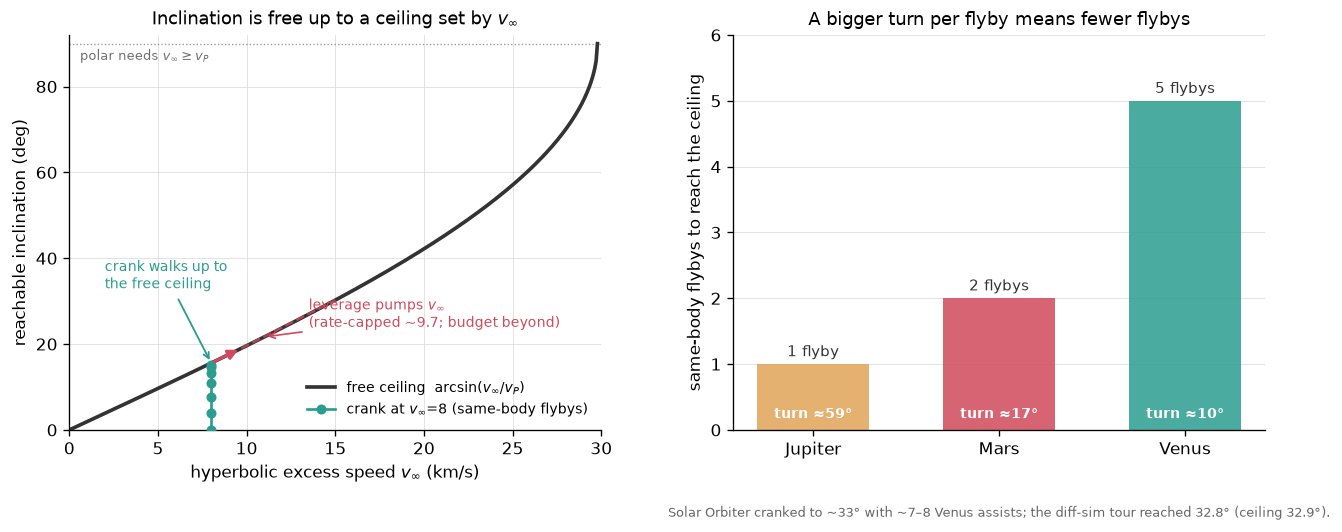
Then the part I wanted to see. Hand the optimizer a target inclination and a fuel-minimizing objective, tell it nothing about cranking or leverage, and seed it at zero leverage. It rediscovers the textbook plan on its own — crank when the target sits under the ceiling (essentially free), and pump the excess speed first when the target sits above it, spending 1.19 km/s where the analytic budget is 1.20. Reaching an inclination this way runs 2–12× cheaper than a direct engine plane change. Same story as the combined burn and the J2 dive: pointed at the fuel bill, it finds the maneuver.
The pump has a catch worth the last figure. Raising the excess speed uses V∞ leveraging — a small burn at the far point of a resonant orbit changes the speed at the next flyby by much more than the burn itself, a factor of 15 to 37 measured against the real ephemeris. Resonant means the spacecraft's period is a whole-number ratio of the planet's, so the planet is back at the meeting point when the spacecraft is. But the same leverage throws the return off the real Earth, and Earth sits in one place, not smeared around its whole orbit the way an idealized model assumes. Inside Earth's sphere of influence, Earth rather than the Sun is the body you fly the trajectory around. Keeping the return inside that sphere caps the pump near 0.085 km/s of excess speed per lap, so a single-planet staircase creeps from excess speed 8 to about 9.7 and then stalls.
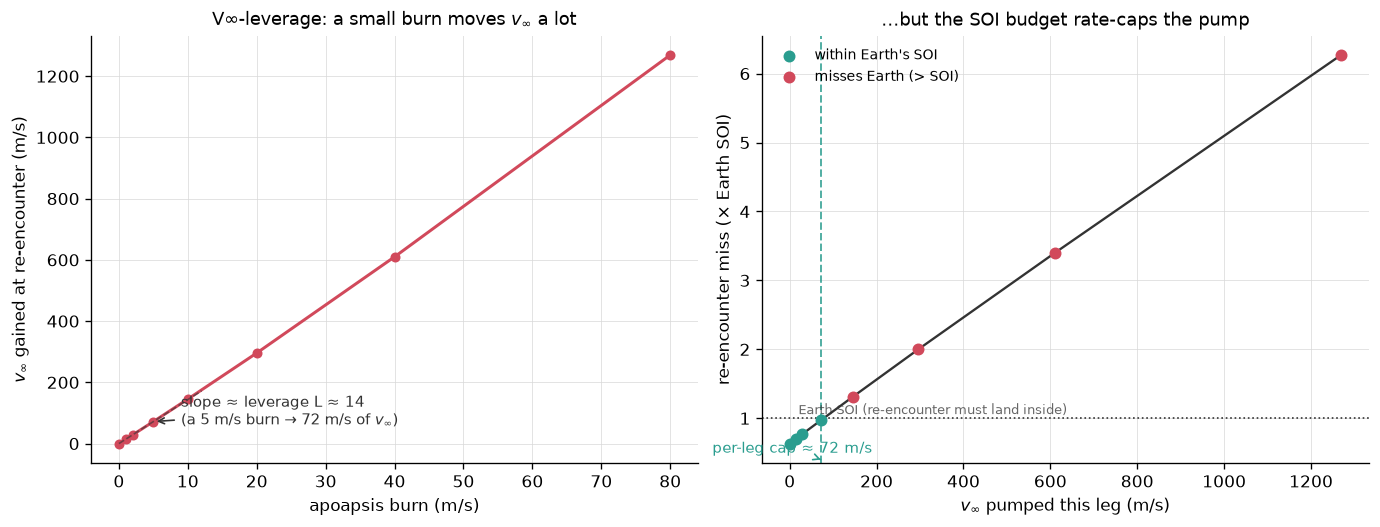
Pinning down why took five pre-registered rounds, each correcting the one before. A naive fixed-resonance staircase looks like it kills the leverage. At the right burn scale the leverage is fine, but rate-capped by the sphere-of-influence budget. The cap isn't a quirk of one resonance: every resonance gives the same 0.1–0.19 km/s per lap. And the obvious fix, bending the flyby, turns out to be mis-timed, because it sets the outgoing orbit before the burn throws off the return, so it can't correct it. The correctly-timed fix does break the cap, but only by trading fuel one-for-one, and the amplification is gone. The cheap way out is a second planet: inner planets pump faster because their years are shorter, and the handoff between planets rides a quasi-conserved quantity (the Tisserand parameter), so it costs nothing.
Making that discoverable by gradients took a reformulation. The obvious differentiable setup solves each leg as a boundary-value problem (Lambert) and penalizes any flyby mismatch. It fails: the resonant-return legs a deep tour needs sit at near-singularities of that boundary-value problem, the gradient there spikes past 10¹⁸, and the optimizer climbs straight into the singularity — reporting huge excess speeds while quietly violating the flyby physics. No amount of gradient clipping or penalty tuning saves it. The fix is structural: propagate each leg forward with a differentiable Kepler propagator (no boundary-value solve anywhere), make the flyby a bounded rotation of the excess-speed vector so its magnitude is conserved exactly (the constraint the optimizer used to cheat no longer exists as a constraint), and hit the real moving planet with a Gauss-Newton solve inside the differentiable loop. The leading legs then close to meters against the real ephemeris, and the trailing resonant returns to well inside the planet's sphere of influence.
The tour that architecture finds: from a 5.95 km/s launch, four pumping flybys of Venus and Earth reach an excess speed of 16.3 km/s — one Earth→Venus handoff is worth +5.0 km/s by itself — with every encounter hit ballistically and no maneuvers at all. Once the pump saturates, five more Venus flybys crank the inclination from 1° to 27.1°, which is 97% of the arcsin(v∞/v_P) ceiling. Counting only the four legs that close tightly it is 92%, since the last of the walk rides loose sphere-of-influence grazes. The crank pays a tax the idealized theory misses: each flyby must also re-hit the real moving planet, and that re-targeting pins about half of every turn, so the walk takes five encounters instead of the ideal one or two. And the epoch matters. Across eight launch epochs spanning two synodic cycles, five pump to 15–18 km/s, two have no viable cheap launch at all, and one launches fine but never climbs: a median of 15.3 km/s across all eight.
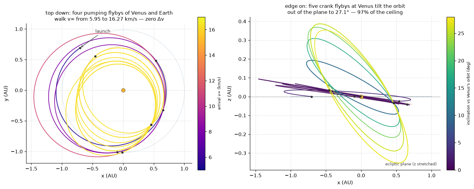
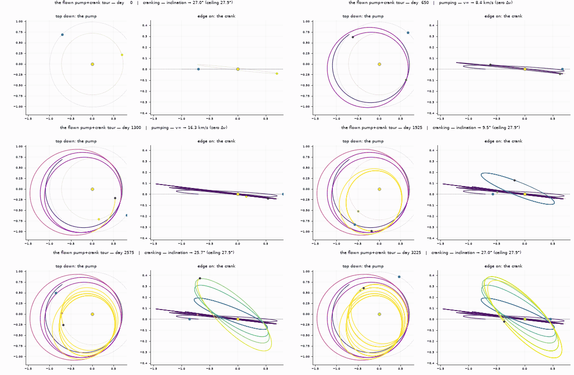
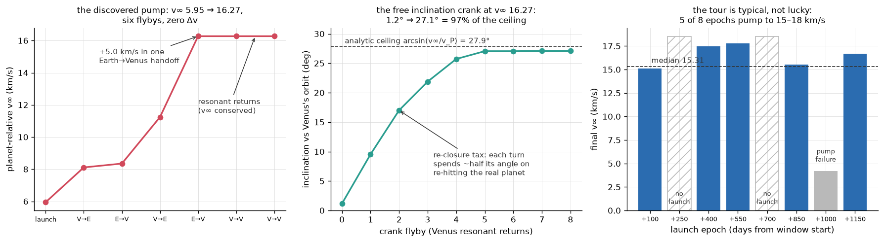
This whole study is patched-conic: every leg is flown as a two-body arc around one body at a time, and each flyby enters as an instantaneous rotation of the excess-speed vector. So it is a claim about the mechanism and not a fuel record. A gravity-assist plane change is cheaper across the board and order-of-magnitude cheaper only when the leverage is favorable, and an agent differentiating through the physics finds the strategy without being shown it.
13. What doesn't work yet
- From-scratch discovery in 3-D is blocked. The exact gradient can refine a competent policy but can't bootstrap one: a policy that never burns gets no signal about when burning would help (the "coast basin"), and there's no exploration mechanism to escape it. Every 3-D result in this report starts from imitation. Stochastic exploration on top of the analytic gradient is the obvious next lever. The version that was tried, reparameterized noise plus an entropy bonus, never escaped the basin, and the one that did work needed a rescaled final layer instead.
- The headline numbers are single-evaluation. 4,096 fresh episodes is a real sample, but it's one sample. The claims discipline (no in-run telemetry, fresh sets only) exists precisely because a single Adam step moves eval success by ±3 points.
- The ephemeris tour is searched and polished, not yet a trained policy. Section 12's pump-and-crank tour is found by tree search over ballistically-closed continuations, with gradients polishing the continuous parameters. The discrete choice of which flyby to take next is still enumeration, not learning. Gradients didn't make that choice in this formulation: zero of five restarts found a valid tour, and they climb into boundary-value singularities when asked to. No full transfer policy has been trained end-to-end on the real ephemeris. The big low-energy wins (permanent capture, Sun-assisted perigee lowering) live here too.
- Eclipse avoidance was refuted. I expected a low-thrust policy to learn to avoid burning in Earth's shadow. It doesn't, even when incentivized: cancelled-in-shadow thrust costs no fuel in the current model, so there's nothing to avoid, and decision-level control is too coarse for shadow arcs anyway. There's nothing to learn here until a binding cost (a deadline, battery mass) exists.
- Real-mission benchmarks are a plan, not a result. A registry of flown missions (MAVEN, Perseverance, Voyager 2, and others) exists for a future comparison via JPL Horizons data. The benchmark doc ends with a warning to my future self: real missions optimize constrained multi-objective problems, and "we beat NASA on Δv" is almost certainly a sign you're measuring the wrong thing.
14. Conclusion
The 2021 report ended with an apology. This one ends with numbers: 92.3% success on the full 3-D task, 1.03× the analytic-optimal fuel at a sister checkpoint that succeeds on 91.9%, a policy that outgrew the oracle that taught it, one rediscovered operational maneuver, one modest verified beat in the three-body regime, and a verification harness I trust more than my own enthusiasm.
The method's scorecard: differentiable simulation, given a competent starting point, refines it past its teacher and matches the provably-optimal solutions wherever they exist — the Edelbaum spiral at 1.006×, the apoapsis burn at 1.03×. Those matches make the other results credible: when the same optimizer, pointed at dynamics with no closed-form answer, produces a combined burn, a dive-drift phasing, or a manifold capture, I believe it because it matched the solved cases first.
The 2021 version of this project wanted to beat Hohmann and never loaded its own model weights. This version knows exactly what it has: a small network, an exact gradient, a verified simulator, and a to-do list of the regimes where beating the textbook is actually possible.
Technical details
- Stack: Python ≥ 3.12 (uv-managed), JAX/XLA for the training hot path, PyTorch reference implementation, NumPy/SciPy, Gymnasium environments, hand-rolled quaternion/orbital/dynamics/attitude libraries (pyright strict, test-covered), astropy/astroquery for JPL Horizons ephemerides.
- Hardware: one RTX 3060 (12 GB). Total policy size: 13→128→128→4, three weight matrices.
- Method: differentiable-simulation policy gradient —
jit(value_and_grad)through full rollouts (~1,200 RK4 substeps, 60 decisions); trimmed-mean + measured-p90-clip gradient aggregation; EMA banking; imitation bootstrap via scripted experts + DAgger. - Verification: fresh 4,096-episode evaluation sets, float64 dt=1s re-flight of 1,024 of them, tolerance-box lower-bound check (0/1024 gamed), RK4 energy audit, pre-registered experiment rounds logged verbatim.
- Everything is public: code, the round-by-round experiment records in the repo docs including the refuted rounds, the checkpoints behind the figures (GitHub release), and the unmodified 2021 code, plots, and reports.